Gradient Descent and Training Process
Table of contents
Introduction
Throughout our exploration of classifiers, we’ve frequently referenced the concept of training. While there are straightforward methods like storing the entire dataset for algorithms like k-NN, these methods are often inefficient. Effective training of classifiers is a complex process that can be extremely costly. For instance, training some of the largest and most well-known neural networks, such as GPT models, can cost millions of U.S. dollars. Understanding the training process is crucial, and the most commonly used training algorithms are based on gradient descent. Gradient descent is an iterative technique used to minimize a loss function.
Loss Function for Training
To enhance our classifier, we need a way to measure its performance. This measurement is provided by a loss function. The loss function takes the logits (the raw prediction scores from the classifier) and the true label of the data as inputs and outputs a single number indicating how well the classifier is performing. The loss function is essential because it guides us in adjusting the classifier’s parameters to improve its performance.
Loss Function A function that evaluates the performance of a classifier. It takes the logits and the true labels as input and returns a single number representing the classifier’s performance. The goal is to minimize this loss function to enhance the classifier’s accuracy.
\[\mathcal{L}(\boldsymbol{s}, \boldsymbol{y}) = \ell, \quad \boldsymbol{s} \in \mathbb{R}^{c}, \quad \boldsymbol{y} \in \mathbb{R}^{c}\]Here the \(\boldsymbol{s}\) represents the logits of the classifier, and the \(y\) represents the true label in one-hot vector form. The loss function outputs a scalar value \(\ell\) that quantifies how well the classifier is performing.
It’s important to note that the loss function typically requires the true label in a one-hot encoded format, which is explained in detail in the Loss Functions section.
Gradient Descent
Gradient descent is a fundamental optimization technique used in training classifiers. It works by iteratively adjusting the parameters (weights and biases) of the classifier to minimize the loss function. The key idea is to compute the gradient of the loss function with respect to the parameters and update the parameters in the opposite direction of the gradient. This iterative process continues until convergence, where the loss function is minimized or a stopping criterion is met.
Key Steps in Gradient Descent:
-
Compute the Gradient: Calculate the gradient of the loss function with respect to each parameter (weight and bias). The gradient indicates the direction and magnitude of the steepest increase in the loss.
-
Update the Parameters: Adjust each parameter in the direction that reduces the loss function. This adjustment is proportional to the gradient and a predefined learning rate, which controls the size of each update step.
-
Iterate: Repeat the process of computing gradients and updating parameters until the loss function converges to a minimum or a stopping condition is satisfied (e.g., maximum number of iterations reached).
Mathematical Formulation
For a parameter vector $\boldsymbol{w}$, the gradient descent update rule is:
\[\boldsymbol{w}^{(t+1)} = \boldsymbol{w}^{(t)} - \alpha \nabla_{\boldsymbol{w}} \mathcal{L}(\boldsymbol{w}^{(t)})\]where:
- $\boldsymbol{w}^{(t)}$ is the parameter vector at iteration $t$
- $\alpha$ is the learning rate (step size)
- $\nabla_{\boldsymbol{w}} \mathcal{L}(\boldsymbol{w}^{(t)})$ is the gradient of the loss function with respect to $\boldsymbol{w}$
Gradient descent is efficient for optimizing complex models with large amounts of data, though it requires careful tuning of the learning rate and monitoring for convergence to avoid issues like slow convergence or overshooting the optimal solution.
Variants of Gradient Descent
While the formula above describes “Batch Gradient Descent” (where the loss is calculated over the entire training set), this is computationally infeasible for large datasets common in robotics (e.g., millions of camera frames). In practice, we use variants:
-
Stochastic Gradient Descent (SGD): The gradient is calculated and parameters are updated for each training sample individually. This is much faster per update but the updates can be very noisy.
-
Mini-Batch Gradient Descent: This is a compromise. The gradient is calculated and updates are performed on small, random batches of data (e.g., 32 or 64 samples at a time). This is the standard approach in deep learning, as it balances computational efficiency with the stability of the gradient estimate.
Forward Pass and Backward Pass
The training process involves two main computations: the Forward Pass and the Backward Pass.
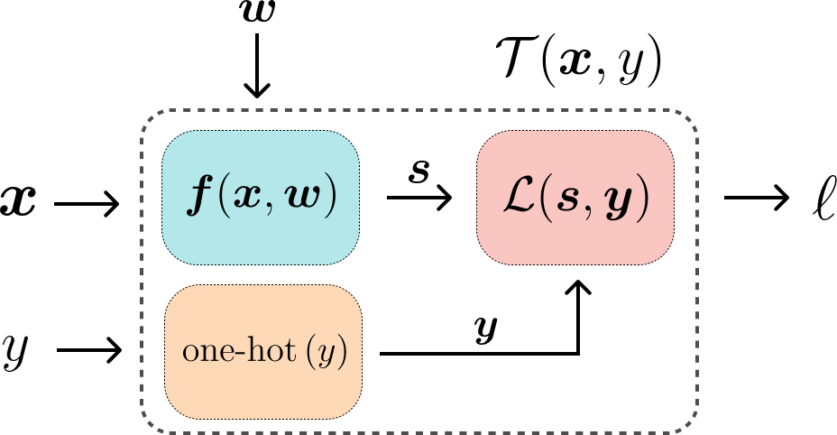
Forward Pass
In the forward pass, the loss is computed given the input \(\boldsymbol{x}\) and the true label \(y\). This is computed using the weights \(\boldsymbol{w}\) as discussed before. Output of the forward pass is the loss \(\ell\).
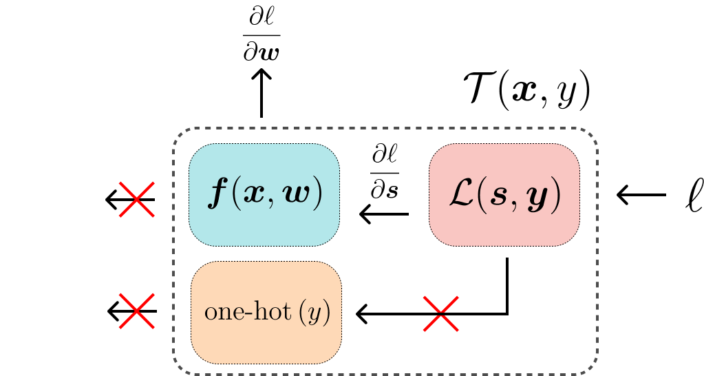
Backward Pass
The backward pass, also known as backpropagation, is where the gradients of the loss function with respect to each parameter (weight and bias) are computed. These gradients guide the updates made to the parameters during gradient descent. The steps involved in the backward pass are:
- Gradient Calculation: Compute the gradient of the loss \(\ell\) with respect to the parameters \(\boldsymbol{w}\).
- Parameter Update: Update the parameters using the gradients. The parameters are adjusted in the opposite direction of the gradient to minimize the loss function.
The gradients are calculated using techniques like the chain rule of calculus, efficiently propagating errors backward through the layers of the model.
Expected Knowledge
Answer the following questions to test your understanding of the gradient descent algorithm.
-
The Role of the Learning Rate: In the gradient descent update rule, what is the purpose of the learning rate \(\alpha\)? Describe what is likely to happen during training if you set the learning rate (a) too high, and (b) too low.
-
The Training Loop: Describe the sequence of steps for one iteration of mini-batch gradient descent. Start with a mini-batch of data and end with the updated model parameters. Clearly define the role of the “forward pass” and “backward pass” in this process.
-
Gradient Descent Variants: What is the fundamental difference between Batch Gradient Descent and Stochastic Gradient Descent (SGD)? Why is Mini-Batch Gradient Descent the most commonly used variant for training large neural networks?