Loss
Table of contents
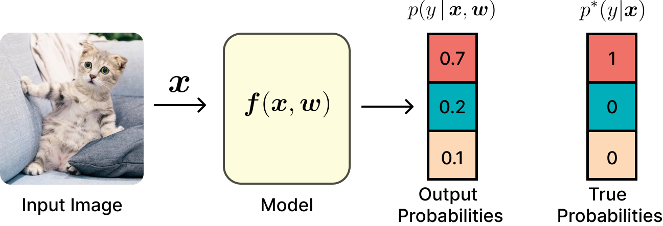
Machine Learning from a Statistical Perspective
In machine learning, we can adopt a statistical viewpoint where \(\boldsymbol{x}\) and \(y\) are random variables connected by an unknown joint probability distribution function \(p^{*}(\boldsymbol{x}, y)\). We can only gather examples \((\boldsymbol{x}, y)\) from this distribution. Our objective is to learn a function \(\mathcal{p}(\boldsymbol{x}, y\vert \boldsymbol{w})\) that approximates the true distribution \(p^{*}(\boldsymbol{x}, y)\), allowing us to make predictions on new, unseen data.
Machine Learning Task: The goal is to approximate the real unknown probability distribution
\[p^{*}(\boldsymbol{x}, y), \quad \boldsymbol{x} \in \mathbb{R}^{d}, \quad y \in \mathbb{N}\]with another probability distribution
\[\mathcal{p}(\boldsymbol{x}, y\vert \boldsymbol{w}), \quad \boldsymbol{x} \in \mathbb{R}^{d}, \quad y \in \mathbb{N}, \quad \boldsymbol{w} \in \mathbb{R}^{m}\]parameterized by \(\boldsymbol{w}\).
Kullback-Leibler (KL) Divergence
To deepen our understanding, we examine the Kullback-Leibler (KL) Divergence.
Kullback-Leibler (KL) Divergence: Denoted as \(D_{\text{KL}}(p \vert\vert q)\), it measures how one probability distribution \(p\) differs from another probability distribution \(q\). For discrete distributions \(p\) and \(q\), the formula is:
\[D_{\text{KL}}(p \vert\vert q) = \sum_{x \in \mathcal{X}} p(x) \log \frac{p(x)}{q(x)}.\]
While this definition might not seem intuitive at first—especially since KL divergence is not symmetric, unlike many distance measures—let’s break it down with an example.
The term divergence implies asymmetry. Unlike metrics, divergences are not required to be symmetric.
Consider a coin with two sides. Define a random variable \(x \in \{0, 1\}\) (heads or tails) and assume the coin is fair, so the probability distribution \(p\) is:
This means the probability of heads or tails is each \(\frac{1}{2}\). Now, consider another distribution \(q\):
To measure how different these distributions are, you might think to simply sum the differences between their probabilities. However, this is not typically how differences between probability distributions are measured in practice.
Instead, consider sampling data from distribution \(p\) and calculating the likelihood of these samples under both distributions \(p\) and \(q\). For example, if we flip the coin ten times and observe:
With five heads and five tails, representing distribution \(p\), we can calculate the probability of these observations under \(p\) and \(q\):
The ratio of these probabilities is:
where \(n_0\) is the number of tails and \(n_1\) is the number of heads. Normalizing and taking the logarithm, we get:
As \(N\) approaches infinity, \(\frac{n_0}{N}\) converges to \(p(0)\) and \(\frac{n_1}{N}\) converges to \(p(1)\), leading to:
This is precisely Kullback-Leibler (KL) Divergence!
The KL Divergence between probability distributions \(p\) and \(q\):
\[D_{\text{KL}}(p \vert\vert q) = \sum_{x \in \mathcal{X}} p(x) \log \frac{p(x)}{q(x)}\]quantifies how “surprised” we would be if samples from distribution \(p\) were claimed to come from distribution \(q\). The smaller the KL Divergence, the more similar the distributions are.
The term Surprisal refers to the amount of information gained, commonly known as Information content or Shannon information.
Understanding the KL Divergence helps us see why it is used in machine learning: we sample data from the distribution \(p^{*}(\boldsymbol{x}, y)\) and measure how surprised we would be if these samples came from the distribution \(p(\boldsymbol{x}, y \vert \boldsymbol{w})\) that we have learned.
Cross-Entropy Loss
Let’s consider our probability distributions within the context of KL Divergence \(D_{\text{KL}}(p^* \,\vert\vert \,p)\).
Thus, minimizing the Cross-Entropy Loss \(H(p^*, p)\) is equivalent to minimizing the KL Divergence \(D_{\text{KL}}(p^* \,\vert\vert \,p)\). This is why we use the Cross-Entropy Loss in practice.
Directly minimizing the Cross-Entropy is challenging because the true distribution \(p^*(y, \boldsymbol{x})\) is unknown. We can approximate it as follows:
where \(\mathcal{D}\) is the dataset and \(N\) is the number of samples in the dataset.
The Cross-Entropy Loss from observed data from the true distribution \(p^*(y \,\vert\, \boldsymbol{x})\) is defined as
\[- \frac{1}{N} \sum_{(\boldsymbol{x}, y) \sim \mathcal{D}} \log p(y \,\vert\, \boldsymbol{x}, \boldsymbol{w})\]where \(\mathcal{D}\) is the dataset and \(N\) is the number of samples in the dataset.
Maximum Likelihood Estimation (MLE)
The Cross-Entropy Loss is closely related to Maximum Likelihood Estimation (MLE). When we use MLE, we aim to find the parameters \(\boldsymbol{w}\) that maximize the likelihood of the observed data. This is equivalent to minimizing the negative log-likelihood of the data, which leads to the same objective as minimizing the Cross-Entropy Loss.
Softmax Function
As previously mentioned, the output of a classifier is a vector of unnormalized scores, or logits, \(\boldsymbol{s}\). To convert these logits into probabilities, we use the softmax function \(\boldsymbol{\sigma}(\boldsymbol{s})\).
The Softmax Function, denoted as \(\boldsymbol{\sigma}(\boldsymbol{s})\), is defined as:
\[\boldsymbol{\sigma}(\boldsymbol{s})_i = \frac{e^{s_i}}{\sum_{j=1}^{c} e^{s_j}}\]where \(c\) is the length of the vector \(\boldsymbol{s}\).
The softmax function takes the logits \(\boldsymbol{s}\) as input and outputs a vector of probabilities that sum to one. This function is used to convert the raw scores output by the classifier into probabilities, representing the model’s confidence in each class and used to make predictions.
Expected Knowledge
From this text, you should understand the following concepts:
- Statistical Machine Learning Task: The machine learning task from the statistical point of view.
- Kullback-Leibler (KL) Divergence: An understanding of the KL divergence between two probability distributions and the intuition behind it.
- Cross-Entropy Loss: The definition and the relationship between the cross-entropy loss and the KL divergence.
- Maximum Likelihood Estimation (MLE): The relationship between the maximizing likelihood estimation and minimizing the Cross-Entropy loss.
- Softmax Function: The definition and why we use the softmax function.